A staged single-node ETL pipeline for terabyte-scale weather data

In 2022 I was handed a problem that looked like a one-liner: take terabytes of raw numerical-weather-prediction (NWP) output and turn it into NumPy arrays a PyTorch training loop can consume. The constraints were the hard part. A single multi-core server, with no Spark or Slurm available. Heterogeneous source models (KIM, UM_N128, UM_N512) with inconsistent grids and known data quirks. An obscure binary format (GRIB2) only one external tool could parse. A hard requirement that training and inference apply exactly the same statistical transforms.

The pipeline I converged on looked like this:

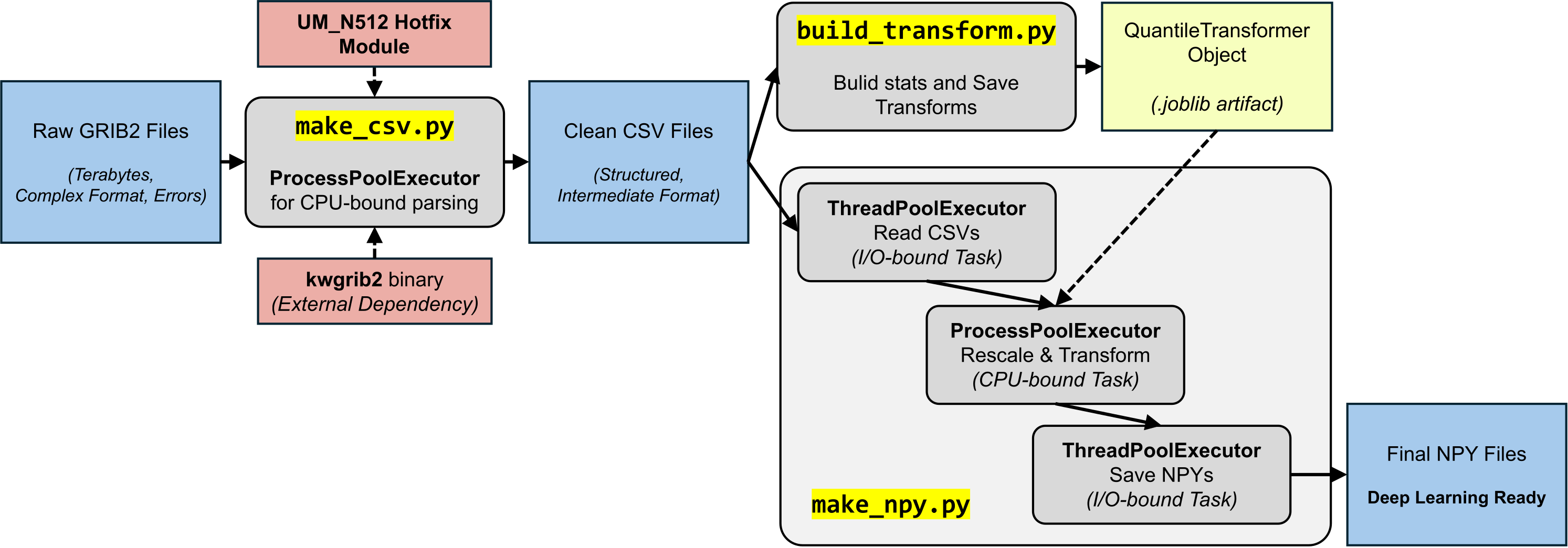
Four decisions are baked into that picture. Each was a real choice with a plausible alternative I rejected.

1. Three discrete stages, not one stream

The forward path goes GRIB2 → CSV → NPY with both intermediates persisted to disk. The streaming alternative (open a GRIB2 file, transform in memory, write the NPY, never materialize a CSV) is what most engineers reach for first.

I went the other way because the intermediates were not waste:

• The CSVs were the canonical “parsed data.” Once they existed, every downstream variation was cheap. Try a different normalization, or generate datasets at a different grid resolution? Re-run only the last stage. A new researcher needed the data in some other format? Hand them the CSVs.
• Stage boundaries were also recovery points. A corrupted GRIB2 file or a NumPy serialization bug only required re-running one stage against the validated outputs of the previous one. With a streaming pipeline, a single bad input poisons the whole run.

The cost is extra disk I/O and storage. For a research workload running dozens of experiments per week, that cost is dwarfed by the cost of re-parsing terabytes of GRIB2 every time someone wants to try a new transform.

A CSV intermediate is not the format I would choose today. Zarr fits this workload better: chunked, compressed, parallel-readable arrays with embedded metadata, exactly the shape NWP fields have. I did not know Zarr existed when I built this. The materialize-intermediates pattern itself still holds; only the format would change.

2. Fit-once, apply-many for the transform

build_transform.py is the small script in the upper branch of the diagram. It fits a QuantileTransformer per variable on a representative subset of CSVs and saves the fitted estimators as a .joblib artifact. make_npy.py then loads that artifact and applies it.

The dotted line in the diagram is the load-and-apply edge. The solid line below it (CSV → make_npy.py forward path) is the data flow. Decoupling these is what makes train/inference parity automatic.

The wrong way to do this (and the way many pipelines do it) is fit_transform() inline at training time. That works exactly until the day you serve a single request and discover your inference path is fitting on whatever it happened to receive. A separate fit step buys three properties:

• Train and inference apply byte-identical transforms.
• The artifact is small, versionable, auditable.
• Re-fitting (e.g., when source statistics drift) is its own runnable step instead of a side effect of training.

3. Pick the executor per stage

Python’s GIL makes “just use threads” wrong for CPU-bound work and “just use processes” wrong for I/O-bound work. Most pipelines I see pick one and live with the loss.

The diagram makes the per-stage choice explicit:

Step	Workload	Executor
GRIB2 parsing	CPU-bound (binary decode + grid math)	ProcessPoolExecutor
CSV read	I/O-bound	ThreadPoolExecutor
Rescale & transform	CPU-bound (NumPy + scikit-learn)	ProcessPoolExecutor
NPY save	I/O-bound	ThreadPoolExecutor

The make_npy.py stage is a thread-process-thread sandwich because it interleaves I/O and CPU. Using ProcessPoolExecutor everywhere would have wasted memory copying CSV chunks across process boundaries when threads handle reads fine; using ThreadPoolExecutor everywhere would have left the CPU stage GIL-bound at single-core speeds.

The rule: measure where each stage spends its time, then pick the concurrency primitive that matches.

4. Quarantine the messy bits

Two boxes in the diagram are colored differently because they were the project’s known risks:

• kwgrib2 binary. An external dependency with no PyPI presence. I wrote a shell script that downloads, patches (adding -fPIC for shared-library compatibility), and compiles it into a known location in the repo, so any team member could provision the environment with one command. Containerization was the next step.
• UM_N512 hotfix module. Archival weather data are noisy in practice. Some UM_N512 files had encoding inconsistencies that didn’t match the spec. The fix lives in code, as an injected module that runs during parsing; it never modifies the source files. Source data stay canonical; the workaround is reviewable.

The pattern in both cases is the same: don’t paper over the messy thing, and don’t bury the fix inside the main script either. Keep it isolated, named, and reviewable, so the workaround is easy to find when the upstream tool changes.

What this generalizes to

Strip the GRIB2 specifics and what’s left is a template for any single-node batch ETL where intermediates are valuable:

Materialize intermediates that double as artifacts. Decouple fit from apply for any learned transform. Pick the executor per stage. Quarantine messy dependencies and data hotfixes into named, isolated modules.

This is not the design for streaming inference, and it is not the design for a true distributed system (the moves change once you have Dask or Spark). It is the design for the much more common case: a single beefy machine, lots of data, and a research workload that will recut the dataset many times before it’s done.